In the intro, I discussed the puzzle of multicellular life: many cell types, one genome. I also followed up by discussing the many statistical issues that arise. There’s a very cool paper from 1999 that brings a lot of clarity to this situation, and here I have space to dig into it a bit.

Akutsu, T., Miyano, S., & Kuhara, S. (1999). Identification of genetic networks from a small number of gene expression patterns under the Boolean network model. In Biocomputing’99 (pp. 17-28). https://www.ncbi.nlm.nih.gov/pubmed/10380182

This paper casts the problem in terms of Boolean network models. These models assume each genes is “on” or “off”, with no other states allowed. The activity of gene A at time t+1 is determined by a Boolean function of other genes. For a made-up example, “Ccl25 is active at time t+1 if, at time t, Foxn1 is active and Gcm2 is not active.” Some papers allows randomness: “Ccl25 is active with 90% probability if at time t, Foxn1 is active and Gcm2 is not active. Otherwise, it is active with probability 0.05.” Surprisingly, this is totally reasonable, even in theory; more below about why.

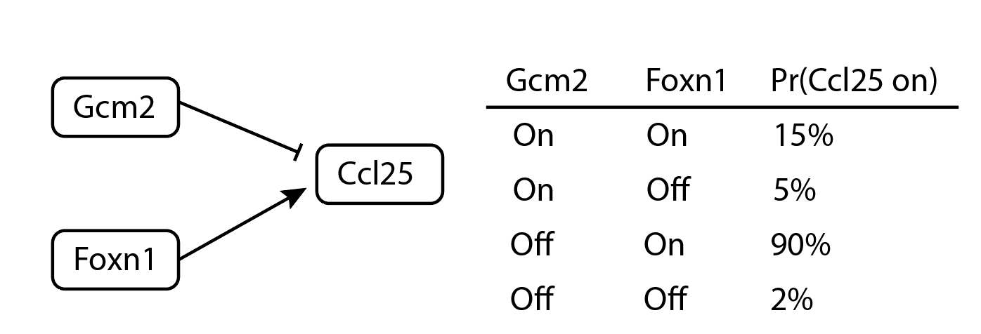
An example of a small probabilistic Boolean network model.

Akutsu et al consider a case where the in-degree is bounded: that is, no gene can be controlled by more that K regulators. How much data does it take to determine those K regulators and the Boolean expression that combines them, for all $n$ genes in the network? Their answer to “how much data” is measured in “state-transition pairs”: each “state-transition pair” is a measurement of cellular state at time t paired with its successor at time t+1. Akutsu et al prove that for a network with $n​$ genes, $O(\log n)​$ state transition pairs are sufficient to identify the original Boolean network.

This is a wonderful and encouraging finding. It suggests that if our consortia or data resources grow at a linear rate, the size of the networks we can successfully study will explode exponentially! Unfortunately, I think most people would agree this explosion hasn’t manifested yet. This is partly due to the “fine print” governing Akutsu et al’s results. First, the scaling with $k$ – the maximum number of regulators per gene – is exponential, i.e. terrible. Increasing $k$ from 3 to 4 or 4 to 5 leads to a massive increase in the amount of data needed. Second, Akutsu et al require that cell states are diverse. Ideally, observations would be sprinkled throughout the state space uniformly at random. This is not what people historically do: most will focus on a narrow domain such as thymocyte development or epithelial to mesenchymal transition. Finally, note that Akutsu et al assume all relevant molecules are measured. In modern genomics, we are still far from simultaneous measurement of all relevant aspects of cell state, and I’ll write more about that here. If we try to average out the effects of unmeasured nodes, then $k$ gets a lot bigger.

Implications

• Let’s start with a concrete number. Quoting Akutsu et al., “The Boolean network of size 100,000 can be identified by our algorithm from about 100 INPUT/OUTPUT pairs if the maximum indegree is bounded by 2.” That’s fantastic! Given an understandably oversimplified model where each gene has up to 2 regulators, we probably have enough data to solve the human transcriptome already! Implementation is left as an exercise to the reader. :P
• The insight about randomly sampling the state space is unsurprising, but it’s also unorthodox. Many existing studies will densely sample a single cell type, process, or developmental trajectory in order to discover regulatory mechanisms specific to that setting. Akutsu et al suggest the opposite strategy: study many diverse cell types.
• Another application of this theory comes when we have to make tradeoffs between the size of a network and the wiring complexity. Here’s an example about a gene whose mRNA (A2) is spliced by gene C into an alternate isoform (A). Downstream, A and A2 have opposite effects on gene B.

Now, you want to model these genes and a bunch of others in a network. Pick your poison:

1. If we count A and A2 separately, we increase the amount of entities we have to relate, and there’s obvious disadvantages. Statistically, you’re adding more useless predictors, which is analogous to increasing the size of the genome in a GWAS.
   • If we count A and A2 only in aggregate, then we can’t predict the activity of B very well: we also have to know whether the splicing regulator C was present when A was being transcribed!

Akutsu et al suggest that option 1 is better. We could double or quadruple the size of a genetic network and we’ll still only need an incremental increase in variety among our datasets. For option 2, we need to permit more complicated predictor functions with more inputs (bigger K). That costs a virtually unlimited amount of data.

Overcoming skepticism of Boolean models

Cells are very obviously not Boolean in nature, and I ordinarily would be uncomfortable with this particular instance of the spherical cow. I had to overcome this skepticism in order to get interested in Akustu et al.’s results.

There are two routes to do so, the first being intuition: biologists are already brimming with Boolean models! When we’re annotating RNA data in the Maehr lab, we almost never ask “Does this have between 10 and 20 transcripts per million of Foxn1?” We ask, “Is Foxn1 expressed?”. Similarly, over-expressing four factors – just turning them from “off” to “on” with no attention paid to the quantities – is sufficient to induce pluripotency. This is one of the biggest breakthroughs in stem cell biology and it’s completely compatible with Boolean thinking.

The other route is through the math. Surprisingly, Boolean models are provably connected to the underlying physics. That’s right: there is a clear line of reasoning to reduce the cell to a Boolean system starting from physical first principles. The derivation has two major pieces, which fit together in sequence.

• In 1977, Daniel Gillespie began with a bath of chemicals, assumed it was well-mixed, and arrived at a Markov process whose mean tendencies followed the types of differential equations that people were already using to model chemical systems. Intuitively, the rate of a given chemical process – such as binding of a transcription factor at a target promoter or formation of a protein complex – should depend on the availability of the ingredients. That’s the core of Gillespie’s argument, and his main contribution is to explain it in rigorous detail. This gets us half way there.
• The other half had already happened four years earlier in 1973. Leon Glass and Stuart Kauffmann figured out how to reduce a simple set of differential equations to a discrete logical system. The Glass & Kauffmann paper allows for a remarkable level of detail, including spatial organization of cells into compartments. They show that Boolean systems can capture the important qualitative behavior of the system. In particular, if a Boolean model predicts that cells can’t traverse a certain path, then the differential equations model should also rule out that path. They could not prove the converse, sadly, but still the Boolean models come close to mimicking the behavior of the much more complex and believeable continuous models.

Together, these papers span from particles colliding in solution to the orderly Boolean models that Akutsu et al study.

Gillespie, D. T. (1977). Exact stochastic simulation of coupled chemical reactions. The journal of physical chemistry, 81(25), 2340-2361.

Glass, L., & Kauffman, S. A. (1973). The logical analysis of continuous, non-linear biochemical control networks. Journal of theoretical Biology, 39(1), 103-129. PDF

Show me more

Another classic on this topic, which I have yet to read fully, is:

D. Cheng, H. Qi and Z. Li, “Model Construction of Boolean Network via Observed Data,” in IEEE Transactions on Neural Networks, vol. 22, no. 4, pp. 525-536, April 2011, doi: 10.1109/TNN.2011.2106512.

If you enjoy super intense Boolean modeling and you want to know what has happened more recently, check out this next paper. Many empirically derived rules are simpler-than-Boolean in certain useful ways: for example, they are often strictly increasing or strictly decreasing in most inputs. This paper takes advantage of that to prune models faster (in terms of the runtime) and better (in terms of the required amount of data). I don’t understand this very well but I think the scaling is ultimately very similar to Akutsu et al’s result.

Schober, S., Kracht, D., Heckel, R., & Bossert, M. (2011). Detecting controlling nodes of Boolean regulatory networks. EURASIP Journal on Bioinformatics and Systems Biology, 2011(1), 6. https://www.ncbi.nlm.nih.gov/pmc/articles/PMC3377916/

The only other relevant model class with substantial results on identifiability is the vector autoregressive model, which has been studied extensively in economics. I’d like to learn more about that, but I’m not expecting it to work well for stem cell biology: in most situations, the long-term behavior of a mildly noisy linear system is too simple to even produce multiple stable states. That means all cells would converge on one cell type during development according to these models. Maybe that would work for yeast, but not for humans. (I see a Far Side caption: “We’re multicellular and it’s time to start acting like it!”)