This is not a standalone post. Check out the intro to this series. This particular post is about the number one limitation in causal network inference: missing layers. In the most common type of experiment, we measure gene activity by sampling RNA transcripts, reading them out, and counting them. We can only guess at:

• protein levels.
• protein modifications. (For example, phosphorylation or cleavage).
• protein complexes. (Is the protein bound to DNA? Is it bound to other proteins?)
• Hormones or signals entering from outside. (For example, testosterone, insulin, or retinoic acid.)
• tiny little RNAs not captured well by vanilla RNA-seq.
• circular RNAs or other RNA’s that might be there in the data, but haven’t yet been catalogued and “tamed” by our processing techniques.
• different isoforms of each gene. (Some techniques can see this, but many widely popular or commercial single-cell RNA technologies cannot see it).
• chromatin state. (Is the DNA at each locus accessible? How is it packaged, marked, and folded in 3D?)
• subcellular localization of each molecule. (Is it in the cytoplasm or the nucleus? MERFISH or similar might be able to answer this for mRNA, but widespread high-throughput techniques circa 2019 cannot.)

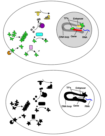
Here’s what this looks like in color versus black and white.

For a concrete example, consider T cell receptor signaling. The T cell receptor goes to the cell surface, forms a complex with several other proteins, binds another molecule outside the cell, opening an intracellular domain to phosphorylation, which recruits a kinase, which phosphorylates a thing, which recruits things that phosphorylate things that hydrolyze things to generate things that promote transcription. I’m not sure what rule I would want infer from just looking at RNA, but it probably contains a lot of AND s!

It’s possible to link measurements from different technologies, especially similar ones like RNA-seq and ATAC-seq. But, this post will consider what most large-scale GRN inference papers do: use mRNA, possibly along with measure of enhancer activity, but nothing else. How should this affect the way we interpret our models? How does it affect our expectations about what we can learn?

Direct binding, direct influence, and indirect influence

I am interested in how stem cells respond to stimuli. So, I want my models to capture causal influence, even if there is no direct physical contact. I also want the models to distinguish between direct and indirect influence: if the effect of A on C can be explained entirely by A==>B==>C, then I don’t want A->C in the model. Unless B is not observed – then I do want A->C in the model! This is the essential criterion: we want direct relationships, not indirect ones, at least to the level of detail that the data permits.

Correct causal inferences aren’t quite enough

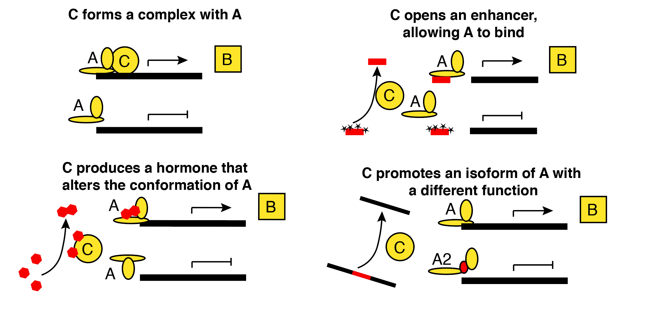
In statistics, we usually confine our anxieties to situations where multiple statistical models or causal models yield the same predictions. In genomics, it can also be useful to consider how different biological models could give rise to the same statistical model. In these situations, statisticians can rest easy, but we still need to lose sleep. Here’s an example of four situations that could lead to the simple rule “Gene B is transcribed when both A and C are present.” Red entities are unobserved in typical 3’ single-cell RNA-seq. Yellow entities represent proteins for which only the corresponding mRNAs are observed.

Cell-state diversity

Most models I have seen do not attempt to explicitly represent missing data. For example, they will not have a count for Foxn1 RNA and a separate count for Foxn1 protein. They just have a single count of “Foxn1”, usually taken to mean the RNA. This greatly simplifies the concepts and the computation, and I’ll follow their lead in this section.

Under this simplification, everything is observed, and I can tell you what most GRN models are doing, at least in spirit.

• Step 1: formulate a complete description of how gene B is regulated. It doesn’t have to be right or even close; it just has to be specific. For example, your hypothesis might state “Genes A and C together completely determine the transcription rate of B with the following formula: dB/dt = 2*A if C>0.”
• Step 2: check if this model is compatible with your observations. If it is, put it on the “maybe” list for gene B. Otherwise, discard it.
• Step 3: make your herd of computers do this over and over until you have tested all hypotheses for all genes. (In practice, people don’t test all models – rather, they implement a variety of computational shortcuts.)

At the end of this process, check the “maybe” list for each gene.

• If it has length 0, you need to consider more flexible models (or better quality data). Try again.
• If it has length 1, congratulations! By process of elimination, and subject to the limitations discussed above, you’ve cracked a tiny piece of the human regulatory code! Pop the champagne.
• If it has length greater than one, welcome to the club: you have an identifiability problem!

The last outcome is most interesting, and it will be a key challenge for the field for the foreseeable future. Often, there’s so much garbage on the list that you can’t do much of what you hoped to do with these models.

This begs the question: what kind of data are needed to get past this issue? And how much? For fully observed networks, this is answered pretty nicely by a cool 1999 paper. I predict the solution to the human interactome will arise very slowly from a combination of 1) observing more and more aspects of cell state and 2) scaling up perturbation assays. In the meantime, it’s possible that the highly flawed results permitted by current data will still be useful for some purposes.