Neural networks are exploding through AI at the same pace as single-cell technology in genomics and GWAS consortia in genetics – that is to say, very quickly. For one example, ImageNet error rates decreased tenfold from 2010 to 2017 (source), but people are also now using neural networks to play StarCraft at a superhuman level, synthesize and manipulate photorealistic images of faces, and yes, also to analyze single-cell genomics data. This seems like a class of models I should consider learning to work with.

Unfortunately, I tried to train a neural net on an image labeling task back in grad school and failed miserably. This left a bad taste in my mouth, and I’d like to start fresh.

Getting started - theory

You don’t need to know any theory at all to start fitting neural networks – see next section. But on the surface of it, neural networks are not complicated compared to a lot of statistical & machine learning methods. A neural net is a just a flexible, tunable function with multiple inputs and (potentially) multiple outputs. It is composed of many sequential transformations:

\(NN(x) = f_n(g_n(f_{n-1}(g_{n-1}( ... f_1(g_1(x)) ... ))))\).

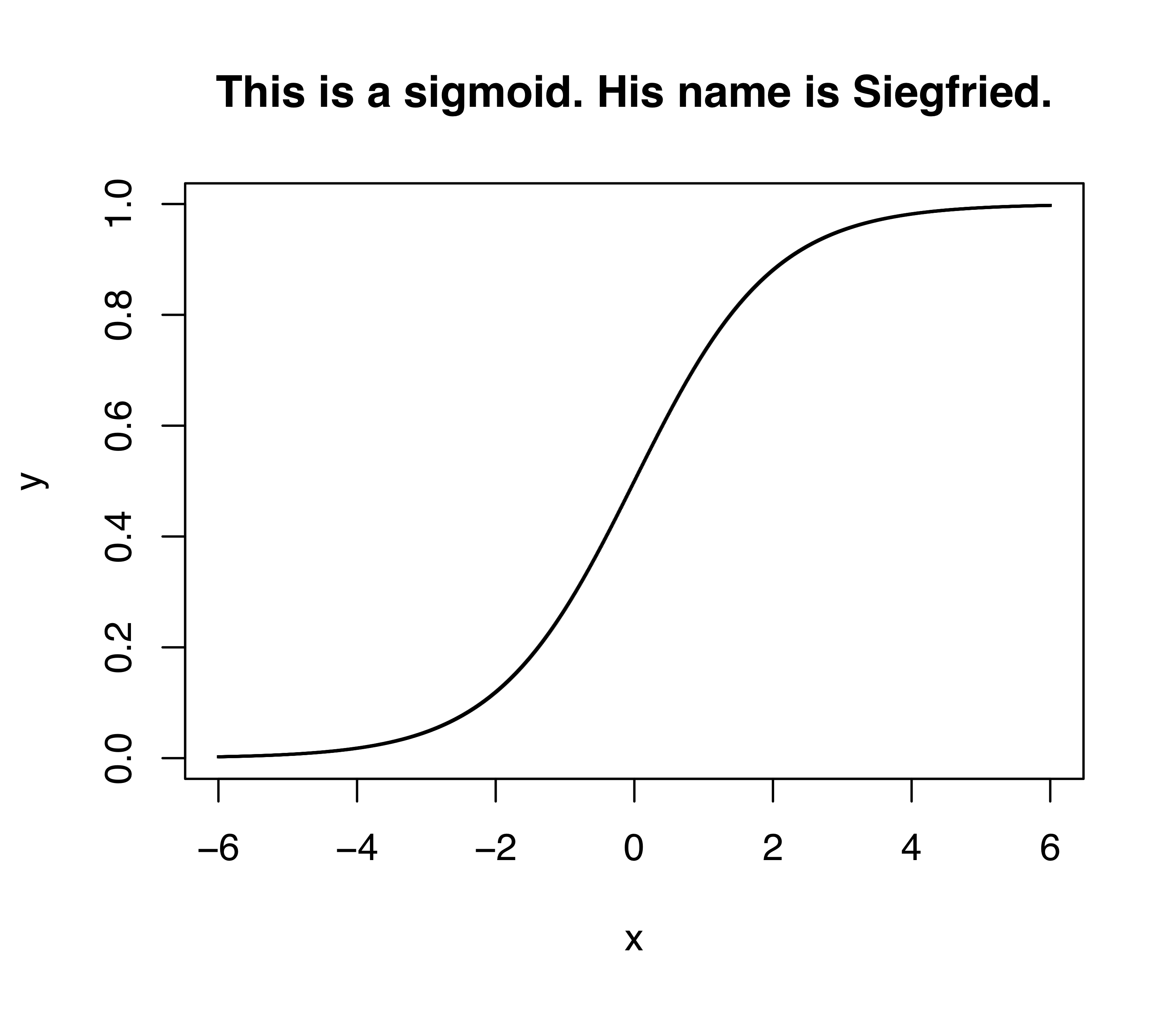
The $g$’s are linear: for example, $g(x_1, x_2)$ might be $5x_1 + 2x_2 + 4$. The $f$’s are nonlinear: for example, $f(x)$ might be a sigmoid $\frac{1}{1+\exp -x}$. Training a neural network just means choosing different values of the parameters: $5x_1 + 2x_2 + 4$ versus $-x_1 + 2x_2 + 1$, for example.

To do the training strategically rather than haphazardly, it helps to take the derivative of the neural net function. This is done using a thing called “reverse mode automatic differentiation” (or autodiff), but autodiff is actually also simple. It’s just a loop that repeatedly applies the chain rule from high school calculus: $\frac{dx}{dy} \frac{dy}{dz} = \frac{dx}{dz}$. The clever part is that it retains certain results as it goes, reusing them instead of starting from scratch at each layer; this speeds things up and saves electricity.

You can fit a neural network without knowing any of this, though: read on.

Getting started - software

I decided to get started using the tensorflow MNIST tutorial for handwritten digit classification. The biggest hurdle was not running the model itself, which was actually a cinch; the problem was the setup. Tensorflow is a very fancy and powerful piece of software: autodiff is easier said than done, and tensorflow implements many additional features such as optimization algorithms and support for different types of hardware. So, it has certain installation requirements. I had to update my operating system twice >︹<. After that, I had a bad time coaxing my notebook to find the installation. (Technical aside: if you’re sloppily following the linked instructions like I did, the trick is that it’s not enough to have the ipykernel package installed globally. It has to be installed in the virtual environment that you are using. Virtual enviromnents contain isolated sets of packages for the Python programming language; here’s what they are and why I use them.)

Once I got that done, the Tensorflow example code ran like a charm.

import tensorflow as tf 
mnist = tf.keras.datasets.mnist
(x_train, y_train),(x_test, y_test) = mnist.load_data()
x_train, x_test = x_train / 255.0, x_test / 255.0
model = tf.keras.models.Sequential([
    tf.keras.layers.Flatten(input_shape = (28, 28)),
    tf.keras.layers.Dense(512, activation = tf.nn.relu), 
    tf.keras.layers.Dropout(0.2),
    tf.keras.layers.Dense(10, activation = tf.nn.softmax)
])
model.compile(optimizer = 'adam', 
              loss = 'sparse_categorical_crossentropy', 
              metrics = ['accuracy'])
model.fit(x_train, y_train, epochs = 1)
model.evaluate(x_test, y_test)

This code reports accuracy in the high nineties after training for a matter of seconds. Tensorflow is very impressive, and I might have had an easier time back in grad school if I had chosen to use it. (At the time, I was using Theano, a similar tool.)

I did a little follow-up to explore the results. This code looks for the most confusing test example – the one where the second best prediction is just about as good as the top prediction.

import seaborn as sns
import pandas as pd
import numpy as np


yhat = model.predict(x_test)
X = pd.DataFrame(yhat)
X['label'] = y_test
X['index'] = X.index

def get_confusion(x):
    y = x.copy()
    y.sort()
    return y[-2]
   
X['confusion'] = np.apply_along_axis(get_confusion, 1, yhat.copy())

sns.scatterplot(data = X, x = 'index', y = 'confusion', hue = 'label')

I added code to print the top five confusing digits so that I could pick my favorite.

X = X.sort_values('confusion')
for image in X.tail().index:
    confusing_digit = sns.heatmap( x_test[image] )
    confusing_digit.get_figure().savefig("confusing_digit" + str(image) + ".png")  

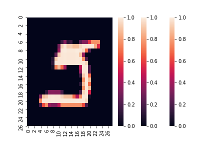
It’s classified as a 5, and as a human, I agree with that, but it’s also the worst 5 I have ever seen.

One hiccup happened when I went to write this up: I re-ran my code and got different images than before! Nondeterministic code makes for bad science, so I added the following four lines from this tutorial to make my output the same every time. (The bad 5 above is part of the final reproducible set.)

from numpy.random import seed
seed(0)
from tensorflow import set_random_seed
set_random_seed(0)

Fortunately, the model is giving very sensible results, even with confusing input, and I can move on to my next tutorial – perhaps reproducing the this paper that analyzes epidermal stem cell development using neural networks. They also use Tensorflow, and they have a lovely public code repository.