This is the fully detailed version of this post about TracerSeq. If you find it daunting, boring, or overly technical, check out the short version first.

---

I recently hosted a discussion in the lab on two Science papers that had sequenced the whole zebrafish embryo at multiple timepoints. Between those two papers, the zebrafish lineage tree is reconstructed using three different datasets and at least four algorithms. The results disagree with each other and with conventional knowledge in fundamental ways. I’m talking about formation of some of the earliest specialized tissues in the embryo – something I assumed was settled long ago. Is the spinal cord seriously part of its own new germ layer, separate from the rest of the nervous system? What’s going on here?

It turns out that there’s actually a fundamental misunderstanding. The technologies used do not all reconstruct the same conceptual “lineage tree”. There are two different kinds of trees. They are related but distinct, and they deserve different names and careful definitions.

I’m not claiming that the authors are confused about this, but it’s subtle, and it’s not spelled out or really even discussed at all in the papers. I bet most readers are confused about this issue.

This blog post attempts to clear things up. I need to start by digging into details of a new technology heavily featured one of the papers. It’s called TracerSeq.

What is TracerSeq?

TracerSeq (paper) is a lineage tracing method: it helps you figure out which cells came from which in the developing embryo.

It’s based on Tol2, which is a naturally occurring transposon from a kind of fish called a medaka fish. (Transposons or “jumping genes” are genes that can copy themselves into new spots in the genome.) Tol2 is a small stretch of DNA – 4.7kb – and it’s really cool because it is modular.

• It’s got sequences that encode a functional transposase protein. Edit these out and there’s no way for it to do its jumping thing – unless you provide transposase separately.
• It’s got little flanking sequences (150 to 200 bases) that allow transposase to recognize it and move it around. Leave these out and it’s just another gene.
• It’s got enough space in the middle to carry up to 11kb of foreign DNA, which is handy for those trying to repurpose it. The essential piece that Wagner et al. inserted is a 20 base-pair random barcode. (For biology geeks, they also put a beta-actin promoter, so that the barcode gets transcribed into RNA and sequenced along with the rest of the regular messenger RNAs that their assay was originally designed to capture.)

When the embryo is still a single cell, Wagner et al. inject a boatload of these randomly barcoded Tol2’s. (I have no clue how they physically do this. Probably magic.) Free-floating barcodes get divvied up by cell division: every time the cell splits, the daughter cells contain a different mix of barcodes. The barcodes also gradually get patched into the genome due to the nature of Tol2. Once a given Tol2 molecule integrates into the genome, the barcode is copied at every cell division, so all the daughter cells share that barcode. You can use shared barcodes to infer shared ancestry between cells. Duuuuuuude.

What do the results look like?

Wagner et al. look at zebrafish embryos from various stages of development leading up to 24 hours. (On a human scale, that’s sort of like 4 weeks. For developmental biologists, it’s at ~30 somites.) The zebrafish has a wide variety of specialized tissues – brain, spinal cord, gut tube, tail bud, epidermis – and the little fishy heart is just starting to beat.

In the first part of their paper, Wagner et al. reconstruct a tree using plain scRNA-seq (no TracerSeq) from various time points. At the final 24-hour time-point, Wagner et al. also sequenced TracerSeq embryos. So, does TracerSeq tell us the same story about how the tissues arise?

No. TracerSeq results actually have little to do with tissue type as determined by single-cell RNA-seq. From the paper:

“Tracer-seq lineage groups tend to be organized by position (e.g., along the [anterior-posterior] axis) rather than strictly by germ layer/tissue origin (e.g., neural, epidermal, mesodermal).”

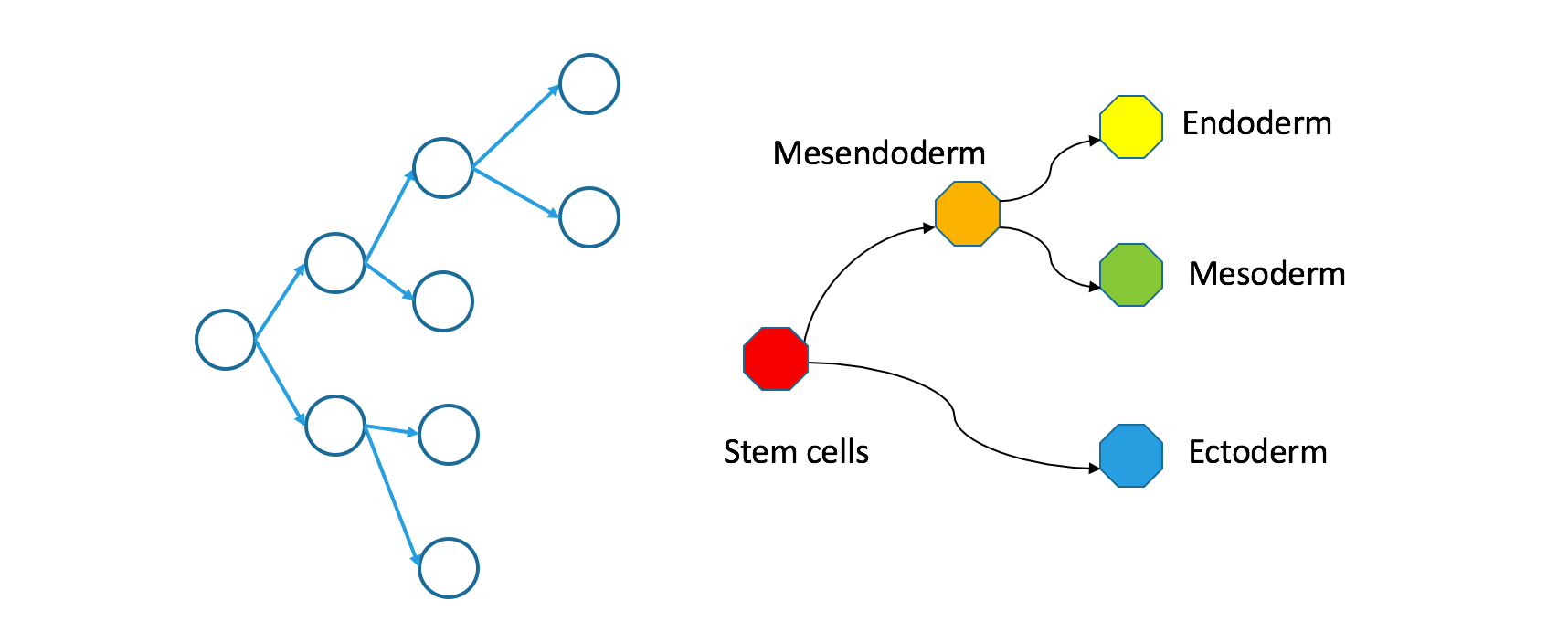
This was a big surprise to me. I’ve never taken a dev bio class, but since joining the Maehr lab, I have absorbed some of the field’s orthodoxy. I thought that the first major split in the lineage tree of any vertebrate would be between the three germ layers: ectoderm gives rise to skin and nerves; mesoderm gives rise to bones, muscles, and the heart; and endoderm gives rise to internal organs such as the stomach, liver, pancreas, and thymus. The TracerSeq results do not follow ectoderm versus mesoderm versus endoderm. They produce a completely different partitioning of the organism!

Clonal trees differ from Waddington trees

In the paper, Wagner et al. ask “how clonal relationships compared with cell state relationships.” When I read the paper, I thought these were two different methods of measuring the same lineage tree. Actually, the underlying trees are related but not exactly the same. Below, I give a formal definition of clonal relationships and state relationships.

Biologists often think about development using a “landscape” metaphor popularized by a man named Waddington. In this metaphor, the landscape corresponds to all the possible states of a cell. In the world of single-cell RNA seq, people might think of it as the set of all possible gene expression patterns. (This leaves out important aspects of cell state – all the dynamic aspects of proteins, DNA, and subcellular spatial organization are missing. But, hopefully it helps you understand what I am saying.) Position on the landscape represents the state of a cell. (Many drawings and discussions of the Waddington landscape reserve one dimension – usually the vertical axis – to measure “developmental potential”, but that is not useful here.)

For this discussion, I’ll define a Waddington tree as the subset of the Waddington landscape that is occupied during natural development, and I will assume it can be discretized into a finite number of states. A typical cell might develop by traversing a path within the Waddington tree. For this discussion, I will assume a Waddington tree has no loops, but my claims can be extended to the case where it is a directed graph with no cycles.

I might also use the term “state-space tree” in place of “Waddington tree”.

The “clonal tree” is much simpler to explain. It’s a binary tree. The root is the zygote (fertilized egg). The children (in the graph-theory sense) are the two daughter cells after this zygote divides. So on and so forth.

In summary:

• For clonal trees, nodes are actual cells. Edges are literal mother-daughter relationships.
• For Waddington trees or state-space trees, nodes are regions within transcriptome space, not actual cells. Edges are pairs of abutting regions.

How do clonal and Waddington trees relate?

Having set out carefully how these two trees are defined and named, it seems obvious that they should relate to each other somehow. Understanding this relationship is key to interpreting the findings the Wagner et al have published.

If you trace a descending path through a clonal tree, it will form a continuous path through the corresponding Waddington tree. That’s true because the Waddington tree includes any state occupied during natural development, and because natural development is effectively continuous.

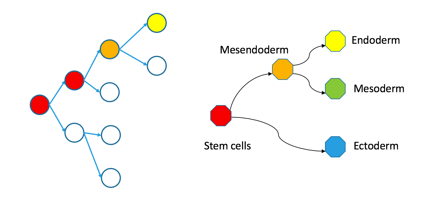
Even though individual cells follow contiguous paths through each tree, the two types of trees are not necessarily superimposable. In an appendix, I define precisely what I mean by superimposability and provide a counterexample. For now, just take a look at my counterexample.

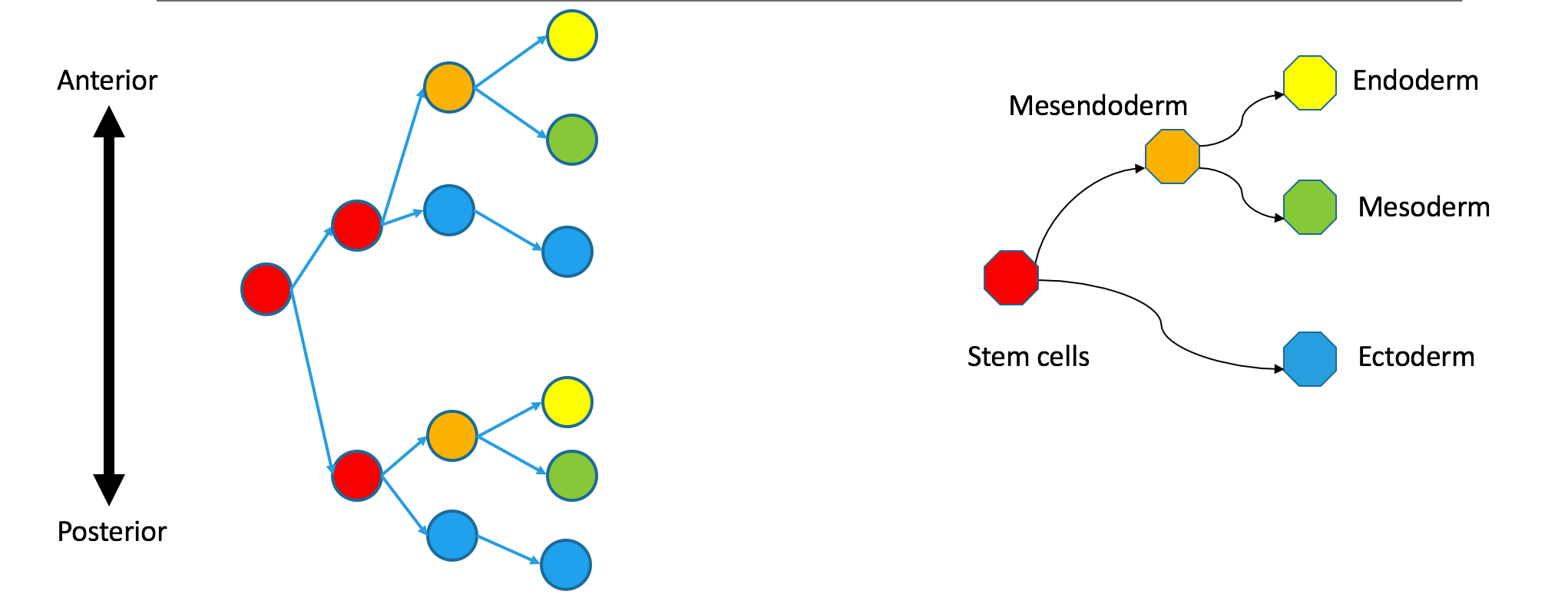
Correspondence between nodes is given by color, with blue mapping to blue, et cetera. The ectodermal subtree of the Waddington tree (the blue node on the bottom right) does not have a single origin in the clonal graph. It contains two separate subtrees of the clonal tree. Biologically, this could happen if the germ layers separated independently in the anterior and posterior parts of the embryo, so the clonal tree does not look like the Waddington tree.

These trees are still biologically compatible. Cells may vary independently in terms of transcriptional identity and clonal origin. An extreme example of this would be to take the two subtrees in the diagram not as anterior and posterior parts of the same embryo, but as monozygotic twins. Their shared clonal tree will have two subtrees that are heterogeneous, each containing many specialized cell-types. (Do zebrafish have twins? I can’t imagine trying to get their names right.)

Observations of this clonal tree should not be taken as evidence against the orthodox view that differentiation begins with the separation of germ layers. They just mean that some clonal separation happens before germ-layer separation.

Bonus material: TracerSeq’s pre-gastrulation emphasis

TracerSeq also tends to amplify the differences between the two types of trees. In the counterexample, recall that the difference arose when cells diverged clonally first, and then diverged in state space. Tracer-Seq tends to emphasize these early clonal divisions that happen prior to divergence along the state-space tree. In the authors’ words,

“… [T]he current timing of TracerSeq integrations encompasses the transition from unrestricted pluripotency to the first fate restriction events appearing in the zebrafish embryo.”

But, I hope I can provide some additional food for thought. The key to my argument is that per-cell Tol2 counts will be cut in half with every cell division. Thus, they will definitely decrease dramatically during development (due to degradation and DNA doubling). By gastrulation, there will be thousands of cells and thus thousands of times fewer integration events per minute for each copy of the genome.

To make this precise, let me consider an oversimplified model of the situation using the following assumptions and notation.

• there are initially $N$ free copies of Tol2
• in each cell, there are $r$ integrations per Tol2 before the next division (with no randomness).
• $N$ is extremely large and $r$ is small, so that losses due to integration are negligible.
• the rate of degradation of Tol2 is negligible.
• mitosis divides the available Tol2 evenly.
• all cells divide simultaneously at even intervals.

After $N$ divisions, a typical cell will contain $rN$ integrations from the single-cell stage, $\frac{rN}{2}$ integrations from the two-cell stage, and so on up to $\frac{rN}{2^{N}}$ divisions from the most recent stage. I am no expert in zebrafish embryo stages, but from a layperson’s reading, the germ layers separate when N is greater than 12. Thus, a little calculation indicates that in any given cell, at any stage of development, more than 99.97% of observed barcodes will have integrated prior to separation of the germ layers. In other words, 99.97% of the barcodes found in each cell will encode information that has little to do with the Waddington tree for zebrafish development.

The quantitative details above are definitely wrong. Later cell divisions ought to happen much more slowly than earlier ones, increasing the amount of time that Tol2 is able to integrate into the genome. I dimly remember that early cell divisions result in a finer partitioning of the human embryo with little increase in volume. If this is true in zebrafish, it could effectively increase the concentration of Tol2 barcodes around each genome, thus increasing the rate of integration at that stage of development. (This makes intuitive sense if we consider only duplication of the genome without the rest of mitosis: the reaction rate would be proportional to $X_TX_G$ where $X_T$ is the concentration of Tol2 and $X_G$ is the concentration of genomic DNA. The reaction rate goes up every time $X_G$ doubles.)

I downloaded the Tracer-seq datasets, and I was planning to back this up with some analysis. Do most barcodes in a given cell actally fall towards the start of the clonal tree? But, the barcode detection is very sparse: of the 1113 tol2 barcodes in clone 1, most appear in 0 cells or 1, and of the 5753 cells, most have no Tol2 barcode or only one. This makes it impossible to infer anything like a complete clonal tree. The analyses that would make the most sense are already in the paper (no surprise): highlighting of partial clonal trees on the Waddington graph (figure 4) and assessment of clonal coupling across germ layers groups (figure 5).

Appendices

Citations

The Tracer-Seq paper

Wagner, D. E., Weinreb, C., Collins, Z. M., Briggs, J. A., Megason, S. G., & Klein, A. M. (2018). Single-cell mapping of gene expression landscapes and lineage in the zebrafish embryo. Science, 360(6392), 981-987.

The other one

Farrell, J. A., Wang, Y., Riesenfeld, S. J., Shekhar, K., Regev, A., & Schier, A. F. (2018). Single-cell reconstruction of developmental trajectories during zebrafish embryogenesis. Science, 360(6392), eaar3131.

Links: Wagner et al, Farrell et al

Graph theory terms

• A directed graph $G$ is a finite set of nodes $N(G)$ and a set of edges $E(G)$. The edges consist of ordered pairs of nodes; each edge connects two nodes. Not all pairs appear; in fact, the edge set may be almost or completely empty.
• A graph is a tree if it is connected and has no cycles. A lack of cycles means for any set of nodes $n_1, n_2, … n_C$ , if the edge set $E(G)$ contains $(n_1, n_2), (n_2, n_3), …, (n_{C-1}, n_C)$ , then it must lack $(n_C, n_1)$. “Connected” means what you think it means: you can move from any node to any other node by following edges.
• A subgraph $G’$ is a graph whose nodes are a subset of $N(G)$ and whose edges are a subset of $E(G)$ containing only edges with both ends in $N(G’)$. Formally, an edge $(n_1, n_2)$ belongs to $E(G’)$ if and only if $n_1$ and $n_2$ are both in $N(G’)$.
• A subtree is a subgraph of a tree that is also a tree.

Superimposing lineage trees

For a precise statement of my argument, I must define what it means to superimpose trees. For readers not trained in graph theory, I will make use of only a few simple concepts. I hope you will be able to read straight through with no problems, but if not, there is an appendix with definitions.

Let a Waddington tree $W$ be represented as a mathematical graph with nodes consisting of lists of numbers (formally, $N(W) \in \mathbb{R}^n$). Suppose for the sake of this discussion that the Waddington tree has no cycles.

Let a clonal tree $C$ be represented as a graph with integers for nodes (formally, $N(C)$ in $\mathbb Z$). Edges $E(C)$ are ordered pairs of mother and daughter cells.

The clonal tree $C$ is defined to be superimposable onto W if each cell state in $W$ arises only once in $C$. Formally, if $S$ is a subtree of $N(W)$, then the corresponding nodes in $S$ must also be a subtree.

In the illustrated counterexample, correspondence between nodes is given by color, with blue mapping to blue, et cetera. The ectodermal subtree of the Waddington tree (the blue node on the bottom right) does not have a single origin in the clonal graph. It contains two separate subtrees of the clonal tree. Biologically, this means that the germ layers have separated independently in the anterior and posterior parts of the embryo, so the clonal tree does not look like the Waddington tree.

Acknowledgements

The better intro and the idea of a short version are due to the very helpful feedback from my brother, Paul Kernfeld. Thanks to everyone who read drafts of this post.