Linkage disequilibrium score regression (LDSC) is a workhorse technique at the intersection of quantitative genetics and functional genomics. The core use of S-LDSC is to detect and quantify functional enrichment of genetic associations; for example, “Are STAT1 binding sites enriched for genetic risk of Crohn’s Disease?” or “Are CNS-specific enhancer regions enriched for effects on psychiatric phenotypes?” or “How much disease risk is mediated by known effects on gene expression?” Unfortunately, LDSC is fairly specialized to a quantitative genetics audience, with derivations using mathematical shortcuts that may not make sense out of context. This series will give a taste of LDSC (rather, five tastes) for the newcomer, including motivation, key formulas, a summary of empirical demos, and a skippable gloss on the derivations.

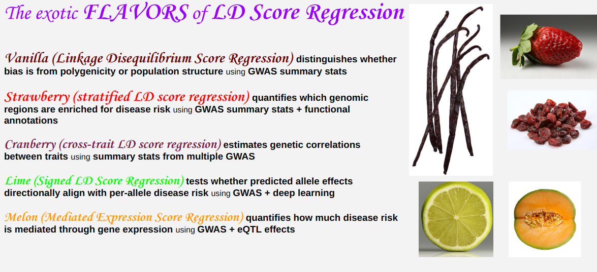
1. this post ---> Vanilla (original LDSC)
2. Strawberry (stratified LDSC)
3. Cranberry (cross-trait LDSC)
4. Lime (signed LDSC)
5. Melon (mediated expression score regression)

Vanilla (the original, Bulik-Sullivan et al. 2015)

I need to walk back my intro for a hot second: with this flavor, we’re just setting the groundwork; this method will not quantify enrichments. Rather, it will diagnose and distinguish between a couple of technical problems. As you’re reading, try to think how you would tell the following two issues apart and quantify them separately.

Confounding by polygenicity

There is a tension in genetic association studies: traits are often influenced by many different loci (they are polygenic), but most studies compute associations with just one locus at a time. In fact, for data privacy reasons, many analysts never get to see the raw genotypes; they only receive summary statistics from single-locus analyses. Furthermore, inheritance is far from independent across loci; human genotypes exhibit linkage disequilibrium (correlation across genotypes). Since there are

1. genotype-genotype correlations that are
2. not controlled for when testing genotype-phenotype correlations,

there are also

1. frequent non-causal correlations between genotype and phenotype.

This effect is not uniform over the whole genome. LD tends to occur in contiguous blocks of DNA. Correlations due to LD thus depend on real effects somewhere physically nearby. Some LD blocks are bigger and some are smaller. Loci in bigger LD blocks will end up with stronger spurious correlations. This is true even if the effects themselves are randomly distributed without regard to position in the genome, which Bulik-Sullivan et al. do assume.

Confounding by population structure

Another mechanism producing “correlation is not causation” is when studies include multiple populations that differ in both genetics and history. For example, in the UK, genotypes reflect fine-grained structure even within Caucasian participants with four UK-born grandparents. Genetic predictions for educational attainment vary strongly on a north-south axis (Fig. 3 of Haworth et al. 2019) even after typical attempts to control for population structure (genotype PC’s and study centers were added as covariates). Nominally, this would represent a signal that people from Plymouth are more biologically driven to seek education compared to people from London; however, the most common interpretation is that this finding is an artifact of population structure.

Most genetic differences between human populations are from genetic drift, meaning they are random rather than systematic. For example, a search for loci under selection in the UK (Mathieson and Terhorst 2022) found only 7 loci and one complex trait under selection, and many of these were expected atypical cases: MHC (NIH intro page), lactase (Wikipedia overview), and skin color (2018 review paper). But by and large, confounding by population structure produces correlations that are similar genome-wide, unlike the correlations due to LD.

The formula

Fit a line to some data, and you can separately estimate both a slope and an intercept. The insight of LDSC is that for the right X and Y axis, confounding by polygenicity shows up as the slope, and population structure shows up as the intercept. Here is a key formula to quantitatively express all of the above, and I’ll explain notation below.

\[E[\chi_j^2] = Nh^2_g\ell_j/M + 1 + aNF_{ST}\]

The left hand side of the formula is a squared association statistic $\chi^2_j \equiv N\hat \beta_j^2$. It comes from your GWAS summary stats $\hat \beta_j$. There is one for each locus; loci are indexed by $j$.

The right hand side contains:

1. N, the number of participants.
2. M, the number of loci, and $h^2_g$, a heritability statistic that can be computed prior to running this procedure. These often appear together in this way to ensure that a twice-as-dense genotyping panel won’t make the model expect a twice-as-heritable phenotype.
3. $\ell_j \equiv \sum_{k}r^2_{jk}$, an LD score that summarizes how much correlation the genotype at locus $j$ has with genotypes at other loci (or itself; k=j is included in the sum). The $r^2$ here is a literal squared Pearson correlation.
4. 1, the number one. If $z$ is standard normal, then $z^2$ is chi-squared with one degree of freedom, and $E[z^2] = Var(z) = 1$. If there were no LD and no confounding, then regression coefficients divided by standard errors would converge to standard normals, and their squares would have expected value 1.
5. $a$, a free parameter estimated by the LD score regression procedure.
6. $F_{ST}$, a commonly used measure of how genetically different two populations are. It is between 0 (pops are identical) and 1 (pops are both fixed for different genotypes). Pritchard’s book has an overview.

Application

They ran LD score regression for about 20 phenotypes, and the results are in this table. They compare to a thing called $\lambda_{GC}$, which measures inflation of chi-squared statistics but does not distinguish between bias from polygenicity and bias from population structure. The intercept term is much closer to 1 than the $\lambda_{GC}$. In other words, most of the bias is explained by polygenicity rather than population structure.

Stay tuned for part 2: strawberry.

The next part of this series is on strawberry (stratified) linkage disequilibrium score regression.

Notes on the derivation of vanilla LDSC

It is here. The derivation begins with no population structure, only LD. It uses typical statistics tactics:

• in general, define theoretical quantities and estimators separately, then do math to see how far the estimator is off; for example $\ell_j \neq \hat \ell_j$ and $r_{jk}\neq \hat r_{jk}$.
• univariate linear regression with standardized features yield the estimator $X^T\phi/N$, since the usual $X^TX^{-1}$ boils down to $1/N$
• law of total variance
• variance is quadratic: $Var(AZ;A) = AVar(Z)A^T$.

Some confusing things to watch out for:

• the phenotype might usually be called “y”, but here it is called “$\phi$”. This is an N by 1 vector. When they write $Var[\phi]$, they mean an N by N covariance matrix, not a scalar; $Var[\phi_i] = Var[\phi]_{i,i}$.
• some $X$’s have a subscript $j$ and some do not. This is important.
• Equation 1.5 is quite specific to a genetics setting; my regression classes did not help without context. Specifically, $X$ and $\beta$ are both random. So it makes sense to write $Var[\phi;X] = Var[X\beta + \epsilon;X] = XVar[\beta]X^T + Var[\epsilon]$.
  • Furthermore, $Var[\beta]$ is the M by M identity matrix because they have already scaled the genotypes $X$ in a way that accounts for a biological expectation: rare variants having bigger expected effects.
  • Further further more more, $Var[\epsilon]$ is normally where I punt and write $\sigma^2$, but here, it’s fully constrained. The genetic and non-genetic variance have to add up to 1, and the proportion of variance that is genetic (the heritability) is known a priori.
• Equation 1.9 seems to omit Equation 1.5’s $N(1 − h^2_g)$ without notice; however, this term vanishes like 1/N and typical modern GWAS N is at least $10^4$.

To add in population structure, the core assumptions are:

• two equal-sized populations,
• separated by genetic drift (no selection),
• with the same LD scores (which are like LD block sizes) within each population. This may not always be appropriate, but it is testable.

The math becomes more involved. The LD scores $\ell_j$ are altered by the population stratification, and the difference in phenotype between populations has both an environmental and a genetic component (although the latter is mean-zero). The parameter $a$ can be interpreted as the mean square difference in phenotype between populations: $a = E[(\phi_1- \phi_2)^2]$.